 |
Welcome to Bug Fest!!
Latest version:
BUGFEST 1, v1.13 (bug1v113.zip) [97k]
[System Requirements]
Eureka! I have found it! I have managed to run a self-balanced simulation with stable predator/prey balances! It won't necessarily do it every time, but things are looking up. And when I say "balanced", I mean that they're not going extinct. Wild swings in proportion (an oscillating balance) are common in this sort of system. I have only done a few long duration tests of the balance (about 3 days or so), but things are looking much better than before. I'm leaving in the code to force minimum populations, but they will now be configurable on the new options menu.
I've been quite pleased with this experiment, even though it did not balance itself the way I would have hoped at first (therefore requiring a few "cheats", which are now optional "failsafes").
Anyway, on with the screenshots...
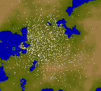
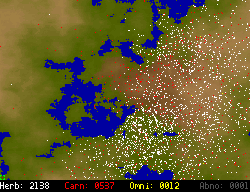
| This shows a typical run with version 1.06. Notice how the predators are slowly pushing the herbivore population along. One of the things that makes this particular scenario interesting is how the whole population was squeezed through a small portion of land between two bodies of water. |
| This picture shows how things often work out a short time into the simulation (in earlier versions). The predators managed to eat most of the herivores that remained in their starting region (which is always the upper-left quarter of the map). This pushed the population more towards the center of the map. The carnivores, as is often the case, spread themselves too thin and thus were unable to breed effectively, and eventually either starved or died of old age, leaving the herbivore population free to grow unchecked. |
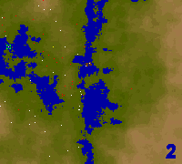
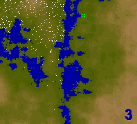
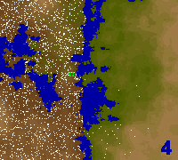
The following sequence of 4 images shows a very interesting situation. By random chance, a very rare sort of map was generated in which the map was divided into two halves by a "river". There were two thin "land bridges" across it, but few bugs discovered this. In shot #1 you can see a fairly normal starting scenario (everyone is in the upper left quadrant). By shot #2, the carnivores nearly wiped out everything, and began to starve. Shot #3 shows the herbivore population on the rebound. That was the last picture taken before letting the simulation run overnight. In the morning I found what you see in shot #4. The population had expanded to fill the entire west side of the map, and they had depleted all of the vegetation (notice the brown color of the land they're on, as compared to the lush green terrain on the east side). They were barely surviving by eating small growths of grass as soon as it would appear.
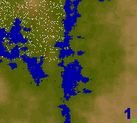 |  |
 |  |
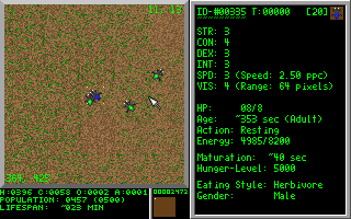
| Here is a screenshot showing the interface at version 1.00 during development. There are several types of background terrain, with different densities of vegetation. This particular shot shows a more arid region, with dry soil and little plant life. Most of the information displayed is straight-forward if you read the documentation. :-) |
|
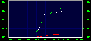
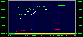
These screenshots show the new population/time graph
that was added in version 1.11. At the time of the
first image, the particular simulation that was running
had only been going for a little over an hour, as you
should be able to tell from the graph. Notice how the
initial population growth is "squished" in the second
image due to the time-compression of the graph. The
entire "plateau" on the right-side of the first image
is squished into the T-1.5 Hour area on the second
image, and it is squished even more around the T-4 Hours
mark in the third.
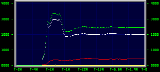
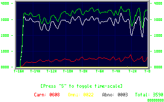
Below is the other time-scale that can be used in the population graphs. The example shows a typical run after nearly 16 hours (simulation time). Notice the population swings that are characteristic of a natural predator/prey balance:
|
|
DOCUMENTATION INDEX |
BugFest runs in DOS (though it is somewhat windows-friendly, meaning running under windows will not fry the system). It requires VGA 320x200x256, and a mouse is recommended. A minimum of 560,000 bytes of DOS RAM is also required.
Welcome to the Bug-Fest! This program was designed mostly for my own enjoyment, but I have decided to make it available for all of you to observe. What it does it quite simple: It simulates a large world complete with growing grass, and lets a whole bunch of simulated insects "live" within this world, eating, breeding, killing, and dying.
My goal was to make a self-sustaining system that would also be interesting to watch. To that end, I have attempted to make the terrain look fairly realistic, and made a few navigational tools (such as the overhead map with mouse-selection of location). Secondly, I was hoping to get a little closer to having a self-balancing system between the predators and the prey, however I feel that generally this is not possible on such a small scale, so I don't feel defeated that this doesn't seem to happen. And of course, the #1 goal was to have fun making it!
In this simulation there are a variety of bugs (when I refer to "bugs" here, I mean "critters" not "program flaws"). The simulation will start with several hundred of them placed within the upper-left quadrant of the map (to give a decent population density for breeding purposes and to give them room to expand into). The map will be generated with a random plasma fractal. This creates a reasonably realistic map, and the data is used to not only determine the color of the soil depending on how far from water it is, but also how much plant life can exist at any given location (also due to distance from water).
The results of the simulation will vary from one run to another. With the same internal settings, I've seen one run end up with all the carnivores dying out and then the herbivores died about an hour or so later while I was away from my computer; And in another run the carnivores managed to wipe out most of the herbivores that weren't on isolated islands. I've also seen the carnivores nearly wipe out the herbivores, but then die because of their isolation from one another (no chance to breed), thus leaving the herbivore population to explode from practically nothing. The balance truly is very dependant on the starting conditions. The lay of the land, the placement of the carnivores relative to one another (if they're too close together they wipe out a region then die of starvation, but if they're too far apart they never breed and all end up dying of old age), and overall food availability all play a part in determining which way it will go. It's almost like a chaos experiment. :-) Of course, after witnessing many such balance swings, I added some code to control the relative population levels to force a little more balance (described in more detail below).
Now, a few specifics...
As herbivores feed, you may actually notice some of the grass disappear near them. Don't worry, it will grow back, though in some places the bugs may eat it faster than it grows (and thus be forced to move on or die of starvation). Each "graphic" change in grass density actually represents 16 individual food units (except for the first step which is only 4), which is why you won't see it change every time. In fact, since all of the critters start the simulation in the upper left quarter of the map, the high density of creatures may result in large patches running out of food completely. You may notice that some bugs will still be able to survive in such regions, simply by eating food the instant it begins to grow back.
Carnivores also grace the landscape, feeding mostly on herbivores, but sometimes also on each other. Unfortunately, it is extremely difficult to obtain a balance between predators and prey in a simulation due to the small scale, and BugFest is no exception. In most runs of this simulation, the predators will die out (though an apparent balance may last a while before this happens), -OR- they may wipe out most of the herbivores then die out themselves afterwards. I don't consider this a failure, just a testament to needing more RAM and a faster computer so that I can have hundreds of thousands of creatures. In fact, an eco-system of herbivores is still an eco-system. The only thing missing from the simulation as such would be to have the grass absolutely require fertilization from the droppings and corpses in order to grow. But my goal was not to make a 100% closed system either. (update: carnivores can never go completely extinct now, due to the "minimum population" code described below; carnivores are necessary to drive the herbivore evolution forward) (update again: it is MUCH more balanced now, and I have seen self-balanced populations arise within BugFest!)
Getting back to eating styles, ocasionally there will be a mutant which will turn out to be an omnivore or that won't eat at all. The omnivores can breed with one another if they find each other, but the abnormals are doomed to die.
In general, the bugs only breed with others of the same eating style (herbivores with herbivores, omnivores with omnivores, etc). When two bugs mate, their stats and traits are passed on to the child. This includes even their pigmentation (red, green, and blue are each passed individually and can come from either parent, hence when blue and red mate, you can get black, red, blue, or purple). When these traits are passed on, there may be slight errors involved (thus allowing for evolution over time as less-effective traits get weeded out). If either the herbivore or carnivore populations drop to less than a certain percentage of each other then the other types will occasionally give birth to the minority type (for instance, there may be 1000 herbivores but less than 10 carnivores, in which case 5% of the critters born to the herbivores will instead be born as carnivores; however if there were 1000 carnivores, but the herbivore count fell below 50, then 5% of those born to carnvivores will come out as herbivores; also, no more than 50% of the population is permitted to be omnivorous). These minimum populations function only as a fail-safe, since the system now seems fairly capable of generating its own balance.
Each of the 6 main stats can be in the range of 1 to 8. The total of the creatures stats is displayed in the upper-right of the tracking window next to the bug's image. This total can not exceed 30. Since there are 6 stats that can each go up to 8, there must be trade-offs and compromises. It will be interesting to see which stats prove to be of the most use to herbivores and which are best for predators.
The stats:
STR: Strength; determines how much damage can be done in an attack. Also slightly affects how much damage the bug can take too.
CON: Constitution; How resistant the bug is to damage, both in terms of how much damage they will resist and in terms of how many "hit points" it will have. This also influences how much energy the bug can store.
DEX: Dexterity; This determines how likely a bug is to hit its opponent, or dodge such an attack. Also slightly influences success at foraging.
INT: Intelligence; Mostly determines success at foraging (particularly when food is scarce), but also helps bugs to not "waste time" trying to mate with infertile or immature females.
SPD: Speed; How fast the bug moves.
VIS: Vision; How far the bug can see. Since they tend to move around a lot, vision range can have a great impact on what the bugs will tend to notice (in terms of being stalked, finding prey, and finding mates, and when fleeing they keep running until they can't see their chaser so obviously if the chaser can see further then they may stop fleeing too soon).
There are a few other traits that can be passed genetically as well, such as color, time to mature, and hunger level.
Hunger level is perhaps one of the more important of these other traits, as it determines when a bug eats. You will see that herbivores tend to keep their energy level very near to their hunger level. Carnivores on the other hand will often be thrown to their maximum energy level after eating, and may not even try to find food again until their energy drops down below their hunger threshold.
Population is controlled in a few ways. First of all there is a hard limit (as of this writing it was 4000, but is subject to change, as it started out at over 5000 but rapidly got cut short due to performance issues, and then was increased a bit again due to some new code added that vastly improved the performance). Secondly, lifespan is shortened proportionately with population. This simulates a limited oxygen supply, and the added propensity for disease in large numbers. To some degree population is also regulated by the predators, though they're unreliable as such in a small scale simulation like this. If by some reason the population does reach the hard limit, then the next child to be born, finding no available "slot" will instead overwrite the oldest living creature. Think of it as a sort of "forced retirement". I've found that the population tends to balance out around 3500. If the population drops below 10 for some reason, a random bug will ocasionally be "spawned" out of nothingness in the upper-left quadrant.
To get started, all you need to do is run the program! When you exit, the simulation will automatically be saved to disk. The next time you run the program, you will be given the option of reloading the saved sim, or starting a new one (which will overwrite the old one).
After the map is created, the simulation will initialize and then it will begin. Details about the simulation are below. However here is a little info about the interface:
Pressing F1 brings up the "about" box.
F2 shows how much DOS RAM is left over.
F3 brings up a help screen.
F4 is the configuration options.
You can use the mouse to select a character for tracking, or you can use the square bracket keys [] to step through the list of critters.
If you don't want to track, you can press enter to turn tracking off, and use the cursor keys to scroll around the map.
"W" changes the "watch mode" which allows you to watch the map display in real-time, or a population graph, instead of the normal tracker-view.
"M" pulls up the map, from which you can select a new location to look at, or you can press the escape key to abort. On the map screen, pressing spacebar will toggle the display of the critters (which are color-coded by eating type, white=herbivore, red=carnivore, etc).
"G" will toggle graphics on/off (turning off graphics allows for faster processing, thus is a good choice if you intend to walk away from the computer and just let it run). When the graphics are off, so is the timing control, so the program will run at maximum speed.
"R" will force a rebuild of the map/bug links. This was added for debugging purposes, but will not harm anything to use. A rebuild is automatically performed periodically anyway.
The escape key quits the program, and automatically saves the current simulation.
WATCH-MODE, Normal:
Just below the viewport is some population data, showing the population breakdown by eating style (c=carnivore, a=abnormal (doesn't eat), etc). There is also a small graph showing the viewport's position relative to the map. This little locator doesn't appear properly centered because its placement is based upon the "maximum" size the map can be, and not the current size. Just above this location graph is a number. This number shows excess CPU time. If the number is 0, then your computer is not keeping up. If the number is not 0, then the program is running at the intended speed. You will see a noticeable change in this number or the program speed as the population increases. Pressing "T" will toggle the timing control. With timing off, the excess CPU time will show as 0 and the program will run as fast as it can. I've found that the excess time drops to zero on my pentium 150 when the population gets over 1500 or 1800 or thereabouts, but doesn't slow down overly much even with 3500 creatures.
The right half of the screen is the information for the bug that you are currently tracking, including stats, health, energy, gender, etc.
WATCH-MODE, Map:
The map mode is fairly self-explanatory. Just like the map that appears upon pressing "M", you see the map, the critters, and the population levels displayed. If you wish to see what the map looks like without the critters, or you want to select a region to zoom in on, or you wish to track a bug, you still need to press "M" for the normal map. In order to see the zoom-in/tracking view, you need to return the watch-mode to Normal.
WATCH-MODE, Graph:
The population graph is displayed such that the vertical axis is population, and the horizontal axis is time. The right-most end of the graph is the current time. Depending on whether you are looking at tyhe linear scale or the exponential scale, the left-most point represents a time approximately 16 or 8 hours in the past, repsectively.
In both graphs, the time scale is based on simulation time, so if your computer is not keeping up with the speed at which the program actually wants to run, you will see that it may take more than 16 hours to reach the 16-hour mark. It was done this way for several reasons- 1) Simplicity, 2) accuracy of the data. Reason #2 allows you to compare data collected on different computers and have a valid comparison.
Linear scale:
The graph displays 16 hours of time, with each pixel
representing 4096 program cycles. This linear scale allows you
to see population swings with enough detail and over a long
enough time period to get a general sense of the population
changes over time.
Exponential scale:
If you look closely, you'll see vertical lines at each of the
time marks. These represent the transitions between the different
zones of the graph. Each zone is updated at a different speed to
achieve the exponential display of time. An easy way to think of
it is that each 32-pixel wide "column" (the space between two
lines) represents the same amount of time as the entire remainder
of the graph to the right of it. For instance, the left most block
represents 4 hours, just as the right-most 7 blocks together also
represent 4 hours. By using this method, you can see a lot of
detail in the most recent population fluctuations, and still get a
general impression of the ones that happened quite some time ago.
If you really like a simulation you've run, and you would like to save it, here's how you do it. Simply rename BUGFEST.SIM to something else. For instance, I ran a really cool simulation that had a river right down the middle of the map, so I saved it as RIVER.SIM. If you want to use the sim again later, just copy it back to BUGFEST.SIM.
This program was written in Turbo Pascal 6.0 (yeah, ok, I'm a dinosaur at heart), with inline assembly language for the graphics and file-handling routines. Due to performance limitations on my pentium, I actually ended up making the maximum population and map sizes smaller than I originally designed (after driving myself nuts about trying to make them as big as possible and being disappointed with the memory space available). For performance reasons, I also opted to not use XMS or EMS or any other method of accessing memory beyond the 640k base DOS Ram.
This first Bug-Fest project took 3 full days to create, though some tweaking, balancing, and bug fixing was done thereafter. A few extra hours of additional work, and I was able to turn a copy of BugFest 1 into the completed "BugFest 2". This "BugFest 2" program was much more speed/time efficient than Bug Fest 1, but wasn't as pleasant to watch and the ecology behaved a little differently. However, I came up with a way to merge the two map techniques, so the "BugFest 2" program was renamed "BugFest 0" and is now considered just an experiment to help me choose the best method to program into the final project. Therefore this program, BugFest 1, is still the main project, and including this "diversion" BugFest took about 5 days to complete (though the last 2 days were "half days").
As usual, there are several reasons for why I chose TP6 instead of C. First of all, this program fits into the shareware/freeware category, so ease and speed of design are much more important than any minor performance gains from optimizations available in a different language. I can think more easily in TP6 than I can in C (primarily because I use it for shareware so much). Since I've been using TP6 for so long for this purpose, I have also built up a large library of functions and routines for graphics, sound, file handling, and so on. Because of this, any time I sit down to write a program I can make one very quickly, as I did with this program. Also, I tend to fix bugs efficiently when I can run the program, change some code, and be running the program again in seconds. TP6 takes less than 3 seconds to compile most of my programs; significantly less in this case due to it's small size. Don't believe me? Look at this:
Turbo Pascal  Version 6.0  Copyright (c) 1983,90 Borland International
BUGFEST.INC(443)
BUGFEST.PAS(1525)
1968 lines, 0.2 seconds, 70352 bytes code, 6642 bytes data.
And for the curious, there is a debug screen you can get to by running the program with the /BUGTEST parameter that shows all of the possible color combinations for all of the bug types.
1.13
1.12
1.11
1.10
1.09
1.08
1.07
1.06
1.05
1.04
1.03
1.02
1.01
1.00
I hope you enjoy this little experiment of mine. It's free, so play with it as much as you like, and give copies to all your friends if you like. It may be copied and distributed freely, so long as no one attempts to make money off of it specifically (though including it in shareware or freeware collections/archives such as the now-common shareware CD's is perfectly fine). This will undoubtedly *not* be the last artificial life experiment of mine, as I seem to keep making a new one every once in a while, but so far this one is by far the most visually stimulating and sports the largest populations yet, and it's also the first one I've made with the intention of releasing publically.
Good luck to you, and may digital life flourish in your processor. :-)
-Bones (aka Ed)